Constructing a VAE-based MNIST number generation Jupyter notebook with emphasis on visualizing latent space
Introduction to Variational Autoencoders (VAE) for MNIST Digit Generation
In this blog post, I will guide you through the process of coding a Variational Autoencoder (VAE) for MNIST digit generation. Our goals are to:
- Explore the latent space using different embeddings
- Analyze neuron activation patterns for each digit
Disclaimer: I don’t have a degree in Computer Science, nor am I an expert coder. This implementation is purely for educational purposes, aimed at learning how to represent symbolic music as a binary matrix based on piano roll representations. While the MNIST dataset differs significantly from symbolic music encoding, it serves as a valuable training ground for understanding general machine learning concepts and various model architectures.
I frequently cross-check my code with ChatGPT and other large language models (LLMs), so the code examples may appear quite generic. Despite this, the code is functional and might be useful to others, which is why I’m sharing it here.
You can find the corresponding notebooks with model weights for different VAE setups in this GitHub Repository.
The requirements.txt file can be found here.
General Information and Resources about VAEs
For a general understanding of VAEs, you can check out the following resources:
- Original VAE paper
- Excellent blog posts I found on the web:
Setting up the Notebook and Dataset
We’ll be programming our VAE setup in PyTorch. Let’s start by setting up our device:
import torch

# Check for GPU availability
if torch.cuda.is_available():
    print("Using GPU:", torch.cuda.get_device_name(0))
else:
    print("No GPU available, using the CPU instead.")

# Define device
device = torch.device("cuda:0" if torch.cuda.is_available() else "cpu")
This is a standard cell that I always use at the beginning to ensure the proper device is selected. By reusing the device variable, we can maintain consistent use of the right device throughout our code.
Next, we’ll set up our dataset loader:
from mnist_loader import load_mnist, plot_sample_images
# Load the MNIST dataset
train_loader, test_loader = load_mnist(num_samples_train=60000, num_samples_test=10000, batch_size=64)
# Plot sample images
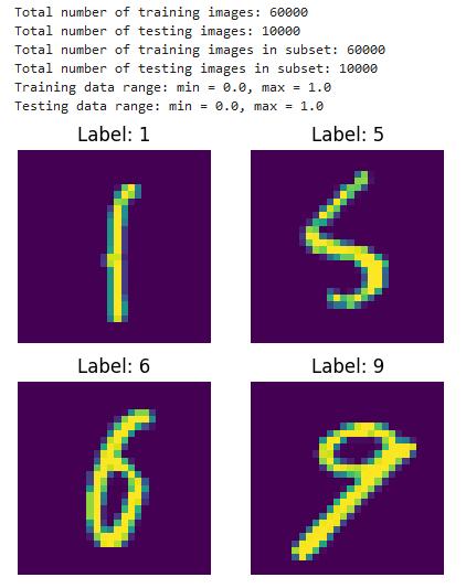
plot_sample_images(train_loader)
Here, we’re using the mnist_loader.py script to download and set up the MNIST dataset locally. You can find the full script here.
I’ve extended the data loader with a set of functions aimed at providing additional information about the size of train and test data within the loaded dataset. It also includes a customized loader where we can define the exact number of images to use during training. This is particularly useful for experiments with very small training sets to see how many features can be extracted (I’ll probably make a dedicated blog post about this in the future).
The loader includes data range printouts to ensure we’re aware of the range of values being fed into the model. Some sample images are also plotted for reference.
Key Features of the Custom MNIST Loader:
- Flexible sample size: Allows specifying the number of samples for both training and test sets.
- Batch size customization: Enables setting the batch size for data loading.
- Data information: Provides details about the size of train and test datasets.
- Value range verification: Prints the range of pixel values in the dataset.
- Visual inspection: Includes a function to plot sample images from the dataset.
This custom loader enhances our ability to experiment with different dataset configurations and ensures we have a clear understanding of the data we’re working with.
Here an example of the output:
Defining the Model
We are going for a conventional VAE model with convolutional and fully connected layers. The Python file with the model can be found here. Below is the corresponding Graphviz plot with latent_dim = 10 (you can find the corresponding notebook here):
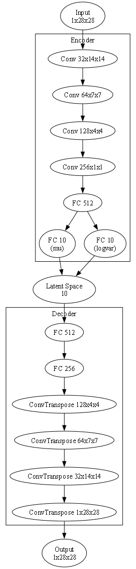
As the model follows the conventional VAE structure, I won’t elaborate on topics such as convolutional/dense layers (an excellent summary can be found here) or the reparameterization trick (you can find excellent sources on it like this or this). Some decisions on the size of the model were made during initial testing, where I found the setup with 256 conv layers and 256=>512 dense layers very stable, especially with low latent_dim values (I couldn’t make a system stable enough for values less than 3 though).
The implementation of kld_weight into the loss function can help with training stability as well and act as a balancing factor between the reconstruction loss (BCE) and the regularization term (KLD). I will definitely explore this topic further in the future (especially the effect of different kld_weight on the training process) but as a rule of thumb:
kld_weight > 1.0:- Increases the importance of the KLD term
- Encourages stronger regularization of the latent space
- May lead to better disentanglement and more structured latent representations
- Can potentially reduce reconstruction quality
kld_weight < 1.0:- Decreases the importance of the KLD term
- Prioritizes reconstruction quality over latent space regularization
- May lead to better reconstructions but potentially less structured latent space
- Can result in less disentangled representations
kld_weight = 0:- Completely ignores the KLD term
- VAE behaves more like a standard autoencoder
- No regularization of the latent space
- May lead to overfitting and poor generalization
kld_weight = 1.0(default):- Balances both terms equally
- Provides a good starting point for many VAE applications
An excellent blog about the effects of different kld_weights can be found here.
Here according loss function implementation:
def loss_function(recon_x, x, mu, logvar, kld_weight=1.0):
    BCE = F.binary_cross_entropy(recon_x.view(-1, 784), x.view(-1, 784), reduction='sum')
    KLD = -0.5 * torch.sum(1 + logvar - mu.pow(2) - logvar.exp())
    return BCE + kld_weight * KLD
Training
Although I am providing the weights for latent_dim = 3, 4, 5, 9, 10, 15, 20, 32 with kld_weight=1.0, you can also train the VAE yourself with the train script (available here) and the following cell:
from vae_training import VAETrainer, LossPlotter

# Assuming model, optimizer, train_loader, and device are already defined
trainer = VAETrainer(model, optimizer, train_loader, device, kld_weight=1.0)
train_losses = trainer.train(epochs=100, log_interval=50)

plotter = LossPlotter()
plotter.plot_losses(train_losses, scale='linear')  # Change 'linear' to 'log' for log scale
I found that training for 100 epochs yielded good results, but due to high loss fluctuations, especially with different kld_weight values, I added an option to show the learning curve plot also in log scale.
Loading the Weights
To load the pretrained model weights, use the ‘vae_model_gauss_enh10.pth’ files and change the number within the file name according to the latent_dim setting:
def load_model(model, path):
    # Check if CUDA is available
    if torch.cuda.is_available():
        # Load the model weights to GPU
        state_dict = torch.load(path)
    else:
        # Load the model weights to CPU
        state_dict = torch.load(path, map_location=torch.device('cpu'))

    # Load the state dict into the model
    model.load_state_dict(state_dict)

    # Set the model to evaluation mode
    model.eval()

    return model

# Example usage
model_path = 'vae_model_gauss_enh10.pth'
try:
    model = load_model(model, model_path)
    print("Model loaded successfully.")
except Exception as e:
    print(f"An error occurred while loading the model: {e}")
I’ve also integrated a dedicated call for CPU-based environments in case you want to run it without a GPU.
Testing the Loaded/Trained Model
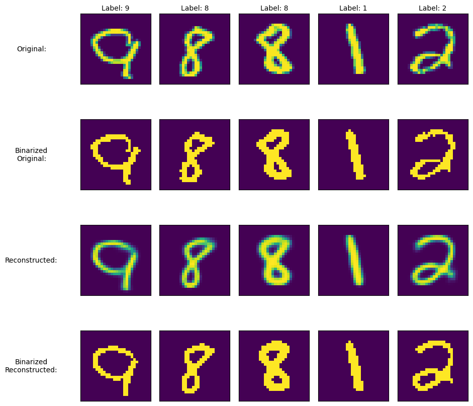
To inspect the functionality of the loaded model, we use some numbers with labels from the loaded test set and reconstruct them with the VAE. Although the MNIST numbers dataset isn’t binary (the inputs for each pixel are set to the range of 0 to 1), I added binary output with a threshold of 0.5 for better visualization of reconstructed patterns within the numbers. I’ve also added a seed to replicate the exact same set of numbers every time the code is run.
Generally:
- When you provide a seed, you’ll get a consistent set of images across different runs or model comparisons.
- When you change the seed, you’ll get a different set of images.
- If you don’t provide a seed, you’ll get a random set of images each time.
import random
import matplotlib.pyplot as plt
import numpy as np

def binarize_image(image, threshold=0.5):
    return (image > threshold).astype(np.float32)

def visualize_results(model, data_loader, num_images=10, device='cuda', seed=None):
    if seed is not None:
        torch.manual_seed(seed)
        random.seed(seed)
        np.random.seed(seed)
        if torch.cuda.is_available():
            torch.cuda.manual_seed(seed)
            torch.cuda.manual_seed_all(seed)

    model.eval()

    # Get all data from the loader
    all_data = []
    all_labels = []
    with torch.no_grad():
        for data, labels in data_loader:
            all_data.append(data)
            all_labels.append(labels)

    all_data = torch.cat(all_data, dim=0)
    all_labels = torch.cat(all_labels, dim=0)

    # Always randomly select indices, but use the set seed if provided
    indices = random.sample(range(len(all_data)), num_images)

    # Get the selected data and labels
    selected_data = all_data[indices].to(device)
    selected_labels = all_labels[indices]

    # Get reconstructions
    with torch.no_grad():  # Ensure no gradients are computed
        recon, _, _ = model(selected_data)

    fig, axes = plt.subplots(4, num_images, figsize=(2 * num_images, 10))
    plt.subplots_adjust(wspace=0.1, hspace=0.5)

    row_labels = ['Original:', 'Binarized\nOriginal:', 'Reconstructed:', 'Binarized\nReconstructed:']

    for i in range(num_images):
        original = selected_data[i].cpu().numpy().reshape(28, 28)
        reconstructed = recon[i].cpu().detach().numpy().reshape(28, 28)

        images = [
            original,
            binarize_image(original),
            reconstructed,
            binarize_image(reconstructed)
        ]

        for j, img in enumerate(images):
            ax = axes[j, i]
            ax.imshow(img, cmap='viridis')
            ax.set_xticks([])
            ax.set_yticks([])

            if i == 0:
                ax.set_ylabel(row_labels[j], rotation=0, labelpad=70, fontsize=10, va='center')

            if j == 0:
                ax.set_title(f"Label: {selected_labels[i].item()}", fontsize=10, pad=5)

    plt.show()

# Example usage
num_images_to_display = 5
seed_value = 42  # Choose any integer value
visualize_results(model, test_loader, num_images=num_images_to_display, seed=seed_value)
As we can see in the rendered test images, the VAE’s reconstructed output has the usual round/blurred edges (here’s an old Stack Exchange thread about blurriness of VAE output: Why is the Variational Auto-Encoder’s output blurred while GAN’s output is crisp?).
We can also clearly see differences within features of the reconstructed images. For example, look at how different the features are within the “9” (first column) in the top right corner, where the circle is connecting to the vertical line:
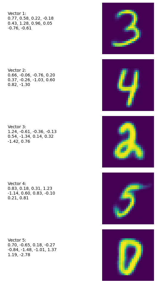
Generating Random Numbers
We can generate random numbers by sampling from a standard normal distribution. In the following example, we use a model with latent_dim = 10, thus representing a point in the latent space as a 10-dimensional vector:
import torch
import matplotlib.pyplot as plt
import numpy as np

def generate_random_numbers(model, num_samples=5):
    latent_dim_size = model.get_latent_dim()
    model.eval()
    with torch.no_grad():
        z = torch.randn(num_samples, latent_dim_size).to(next(model.parameters()).device)
        samples = model.decode(z).cpu()

    fig, axs = plt.subplots(num_samples, 2, figsize=(8, 2*num_samples))

    for i in range(num_samples):
        # Left column: vector description
        vector_str = "Vector {}:\n".format(i+1)
        for j, val in enumerate(z[i].cpu().numpy()):
            vector_str += "{:.2f}".format(val)
            if (j+1) % 4 == 0:  # New line every 4 numbers
                vector_str += "\n"
            elif j != len(z[i])-1:
                vector_str += ", "

        axs[i, 0].text(0.5, 0.5, vector_str, wrap=True, fontsize=10)
        axs[i, 0].axis('off')

        # Right column: rendered image
        axs[i, 1].imshow(samples[i].numpy().reshape(28, 28), cmap='viridis', origin='upper')
        axs[i, 1].axis('off')

    # Adjust the layout to bring columns closer together
    plt.tight_layout()
    plt.subplots_adjust(wspace=0.1, hspace=0.1, top=0.95)
    plt.show()

# Generate and visualize random numbers
generate_random_numbers(model, num_samples=5)
The output looks like this:
Exploring the Latent Space
Based on the previous cell with standard normal distribution sampling, we can modify our inputs to be not simply randomized, but to use controllable sliders with a set min/max range. This allows us to influence the generated outcome interactively within Jupyter:
import torch
import matplotlib.pyplot as plt
from ipywidgets import interact, FloatSlider, VBox, HBox
import ipywidgets as widgets

def create_vae_explorer(model):
    model.eval()
    latent_dim_size = model.get_latent_dim()

    def update_image(**z_values):
        z = torch.zeros(1, latent_dim_size)
        for i, val in enumerate(z_values.values()):
            z[0, i] = val

        with torch.no_grad():
            z = z.to(next(model.parameters()).device)
            sample = model.decode(z).cpu()

        plt.figure(figsize=(4, 4))
        plt.imshow(sample[0].numpy().reshape(28, 28), cmap='viridis')
        plt.axis('off')
        plt.show()

    sliders = {f'z{i}': FloatSlider(min=-3, max=3, step=0.1, description=f'z{i}')
               for i in range(latent_dim_size)}

    interact_manual = interact(update_image, **sliders)

    return interact_manual

# Usage:
# Assuming you have already loaded your model:
# from enhanced_vae_model import EnhancedVAE, loss_function, init_model
# model, optimizer = init_model(latent_dim=10, device=device)
# model = load_model(model, 'vae_model_gauss_enh10.pth')

# Then you can create and display the explorer:
explorer = create_vae_explorer(model)
display(explorer)
This approach allows us to test and understand the influence of every neuron on the final number generation. By adjusting the sliders, we can observe how changes in each dimension of the latent space affect the generated output:
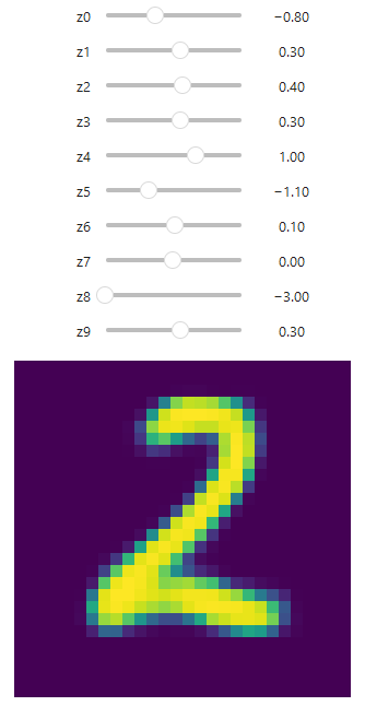
Key Insights from Latent Space Exploration
- Dimensionality: With a 10-dimensional latent space, we have 10 sliders to manipulate. Each slider corresponds to a dimension in the latent space.
- Range: The sliders are set to a range of -3 to 3, which covers most of the standard normal distribution (about 99.7% of the data falls within three standard deviations of the mean).
- Continuous Generation: As you move the sliders, you’ll notice that the generated images change smoothly. This demonstrates the continuous nature of the latent space.
- Feature Control: Different dimensions often control different features of the generated digits. For example, one dimension might control the thickness of the strokes, while another might influence the curvature.
- Interpretability: While some dimensions might have clear interpretable effects (like controlling the loop size in digits like 6 or 9), others might have more subtle or combined effects.
- Interpolation: By moving between two points in the latent space, you can observe how the model “morphs” one digit into another, providing insights into how the model represents the space of digits.
Mapping the Latent Space with Test Dataset
Now that we have some grasp on how our latent space is working, we can try to gather the latent_dim profiles for every number. We’ll do this by sending our test dataset into the model and looking at the exact activation values for every digit. First, we need to save all the gathered vector values into a pandas DataFrame:
import numpy as np
import pandas as pd
from tqdm.notebook import tqdm

def extract_latent_activations(model, data_loader):
    device = next(model.parameters()).device  # Get the device from the model
    latent_dim = model.get_latent_dim()  # Get the latent dimension from the model
    model.eval()
    activations = []
    with torch.no_grad():
        for data, labels in tqdm(data_loader, desc="Extracting latent activations"):
            data = data.to(device)
            mu, logvar = model.encode(data)
            latent_space = model.reparameterize(mu, logvar)

            for i in range(len(labels)):
                digit = labels[i].item()
                latent_rep = latent_space[i].cpu().numpy()

                # Add overall latent representation
                activation_dict = {
                    'Digit': digit,
                    'Latent Representation': latent_rep
                }

                # Add individual neuron activations
                for j, activation in enumerate(latent_rep):
                    activation_dict[f'Latent Neuron {j}'] = j
                    activation_dict[f'Activation {j}'] = activation

                activations.append(activation_dict)

    return pd.DataFrame(activations)

# Extract latent activations
df = extract_latent_activations(model, test_loader)

# Display the first few rows of the DataFrame
display(df.head())

# Basic statistics of the activations
display(df.describe())

# You might want to save this DataFrame for further analysis
# df.to_csv('latent_activations.csv', index=False)
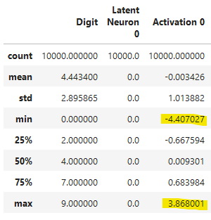
With display(df.describe()), we can clearly see the activation boundaries for every neuron:
Now we can calculate the average neuron values for every digit, generating number prototypes:
import matplotlib.pyplot as plt
import seaborn as sns
import torch
import pandas as pd
import numpy as np

def calculate_digit_prototypes(df):
    # Extract the activation columns
    activation_columns = [col for col in df.columns if col.startswith('Activation')]

    # Compute average activations per neuron per digit
    prototypes = df.groupby('Digit')[activation_columns].mean()

    # Rename columns to match the original format
    prototypes.columns = [f'Neuron {i}' for i in range(len(activation_columns))]

    return prototypes

def generate_prototype_images(model, prototypes):
    device = next(model.parameters()).device  # Get the device from the model
    model.eval()
    with torch.no_grad():
        # Convert prototypes to tensor
        prototype_tensors = torch.tensor(prototypes.values, dtype=torch.float32).to(device)

        # Generate images
        generated_images = model.decode(prototype_tensors).cpu().numpy()

        # Plot the generated images
        fig, axes = plt.subplots(2, 5, figsize=(10, 6))
        for i, ax in enumerate(axes.flat):
            ax.imshow(generated_images[i].reshape(28, 28), cmap='viridis')
            ax.set_title(f"Digit {i}")
            ax.axis('off')

        plt.suptitle("Generated Digit Prototypes", fontsize=16)
        plt.tight_layout()
        plt.show()

# Calculate prototypes
prototypes = calculate_digit_prototypes(df)

# Display the prototypes as a heatmap
plt.figure(figsize=(10, 8))
sns.heatmap(prototypes, cmap='viridis', center=0, annot=False, fmt='.2f')
plt.title('Prototype Neuron Activations for Each Digit')
plt.ylabel('Digit')
plt.show()

# Generate and display prototype images
generate_prototype_images(model, prototypes)

# Print the prototype values for each digit in the specified format
for digit in range(10):
    print(f"Digit {digit}:")
    print(f"neuron_values = {{")
    for neuron_index, (neuron, value) in enumerate(prototypes.loc[digit].items()):
        print(f"    {neuron_index}: {value:.6f},")
    print("}\n")
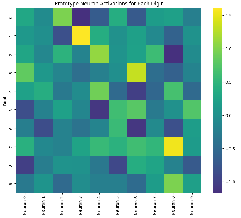
Now we can see the activation heatmap for every neuron depending on a certain number:
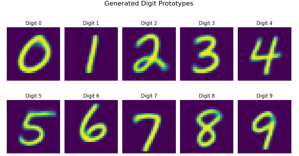
As well as render the “perfect” digit activations based on average neuron values:
Interpreting the Results
-
Activation Boundaries: The
df.describe()output shows us the range and distribution of activations for each neuron across all digits. This gives us an idea of how much each neuron contributes to the overall representation. -
Neuron Activation Heatmap: This visualization allows us to see which neurons are most active for each digit. Brighter colors indicate higher activation. We can observe that different digits have distinct patterns of neuron activations.
-
Digit Prototypes: These images represent the “ideal” or average representation of each digit in the latent space. They’re generated by using the mean activation values for each digit.
Neuron Specialization and Feature Mappings
By examining the heatmap we created earlier alongside the prototype images, we can begin to hypothesize about the features each neuron might be encoding. To gain a deeper understanding of the specific features controlled by each neuron, let’s create a dedicated feature map as a grid image. We can use either a random neuron preset or, for example, take values from one of our previously calculated digit prototypes:
import matplotlib.pyplot as plt
import torch
from torch.distributions import Normal

def generate_images_with_neuron_progression(model, neurons_to_iterate, neuron_values, num_images=16, steps=11, start_value=-2, end_value=2):
    device = next(model.parameters()).device  # Get the device from the model
    model.eval()
    with torch.no_grad():
        dist = Normal(0, 1)

        if neurons_to_iterate is all:
            neurons_to_iterate = list(neuron_values.keys())
        elif not isinstance(neurons_to_iterate, list):
            neurons_to_iterate = [neurons_to_iterate]

        num_neurons = len(neurons_to_iterate)
        fig, axes = plt.subplots(steps, num_neurons, figsize=(num_neurons*2, steps*2.5))  # Increased figure height

        # Ensure axes is always a 2D array
        if num_neurons == 1:
            axes = axes[:, None]

        for step in range(steps):
            z = dist.sample((num_images, model.get_latent_dim())).to(device)

            for neuron, value in neuron_values.items():
                z[:, neuron] = value

            iterated_value = start_value + (end_value - start_value) * step / (steps - 1)

            for col, neuron_to_iterate in enumerate(neurons_to_iterate):
                z_neuron = z.clone()
                z_neuron[:, neuron_to_iterate] = iterated_value

                generated_images = model.decode(z_neuron).cpu()

                ax = axes[step, col]
                ax.imshow(generated_images[0].squeeze(), cmap='viridis')
                ax.axis('off')
                ax.set_title(f"N{neuron_to_iterate}={iterated_value:.2f}", fontsize=8)  # Reduced font size

        manipulated_info = ", ".join([f"N{n}={v:.2f}" for n, v in neuron_values.items()])
        plt.suptitle(f"Neuron Progression\n(Fixed: {manipulated_info})", fontsize=12, y=1.02)  # Added line break and adjusted y position

        plt.tight_layout()
        plt.subplots_adjust(top=0.999)  # Adjust top margin
        plt.show()

# Example usage:
neuron_values = {
    0: 0.286409,
    1: -0.116093,
    2: 0.454476,
    3: -0.171823,
    4: 1.083852,
    5: 0.051394,
    6: 0.222545,
    7: 0.601464,
    8: -1.161078,
    9: -0.070922,
}
neurons_to_iterate = all  # Use 'all' to iterate over all neurons in neuron_values, a single neuron number or a list can be used as well
start_value = -4.5  # Start of the range
end_value = 4.5  # End of the range
generate_images_with_neuron_progression(model, neurons_to_iterate, neuron_values, num_images=1, steps=10, start_value=start_value, end_value=end_value)
Now, we get the following image, where I used the prototype of number 2 as an example:
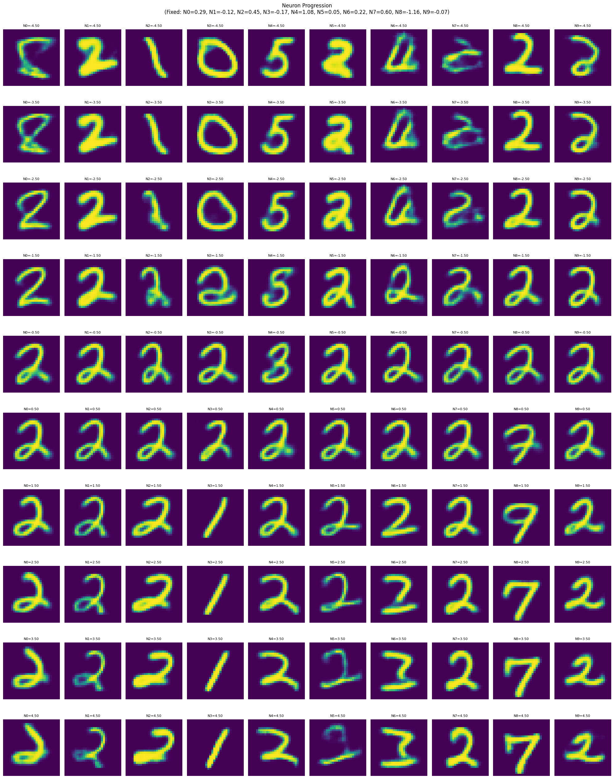
With this visualization, we can clearly see the features controlled by different neurons:
- While some neurons are responsible for one or multiple features (e.g., thickness controlled by neurons 1 and 5, rotation by neurons 1, 2, 3, and 5), several neurons are responsible for more obscure features. For instance, the “curl” in the bottom left corner is influenced to some extent by all neurons, but is particularly evident in neurons 1, 7, 8, and 9.
- Particularly interesting are the “morphing” features, where a certain element is rotated or displaced until a new number becomes recognizable. For example, neuron 3 demonstrates a morphing from 0 to 2 to 1 by folding/rotating the shape.
To visualize the relationship between two neurons within the manifold representation, we can iterate within a certain value range. We need to flip the y-axis because imshow by default places the origin (0, 0) at the top-left corner, but we want to use Cartesian coordinates instead:
import torch
import torchvision.utils as vutils
from torch.distributions import Normal
import matplotlib.pyplot as plt
def generate_2d_manifold(model, neuron1, neuron2, neuron_values, num_images=16, steps=11, start_value=-2, end_value=2):
model.eval()
with torch.no_grad():
dist = Normal(0, 1)
images = []
for value1 in torch.linspace(end_value, start_value, steps):
row_images = []
for value2 in torch.linspace(start_value, end_value, steps):
z = dist.sample((num_images, model.latent_dim)).to(device)
for neuron, value in neuron_values.items():
z[:, neuron] = value
z[:, neuron1] = value2
z[:, neuron2] = value1
generated_image = model.decode(z)
row_images.append(generated_image[0])
images.extend(row_images)
# Create a grid of images
grid = vutils.make_grid(images, nrow=steps, normalize=True, scale_each=True)
# Convert to numpy for matplotlib and apply colormap
grid_np = grid.cpu().numpy().transpose((1, 2, 0))
grid_np = plt.cm.viridis(grid_np[:, :, 0]) # Apply viridis colormap to first channel
# Display the grid
fig, ax = plt.subplots(figsize=(12, 12))
im = ax.imshow(grid_np, extent=[start_value, end_value, start_value, end_value])
# Set labels and title
ax.set_xlabel(f'Neuron {neuron1}')
ax.set_ylabel(f'Neuron {neuron2}')
ax.set_title(f'2D Manifold Representation\nNeurons {neuron1} and {neuron2}', fontsize=16)
# Add ticks
tick_positions = torch.linspace(start_value, end_value, 5)
ax.set_xticks(tick_positions)
ax.set_yticks(tick_positions)
ax.set_xticklabels([f'{x:.2f}' for x in tick_positions])
ax.set_yticklabels([f'{y:.2f}' for y in tick_positions])
# Add colorbar
# plt.colorbar(im, ax=ax, label='Pixel values')
plt.tight_layout()
plt.show()
# Example usage:
neuron_values = {
0: 0.286409,
1: -0.116093,
2: 0.454476,
3: -0.171823,
4: 1.083852,
5: 0.051394,
6: 0.222545,
7: 0.601464,
8: -1.161078,
9: -0.070922,
}
# Select two neurons to visualize
neuron1 = 3 # Change this to your desired neuron
neuron2 = 4 # Change this to your desired neuron
start_value = -4
end_value = 4
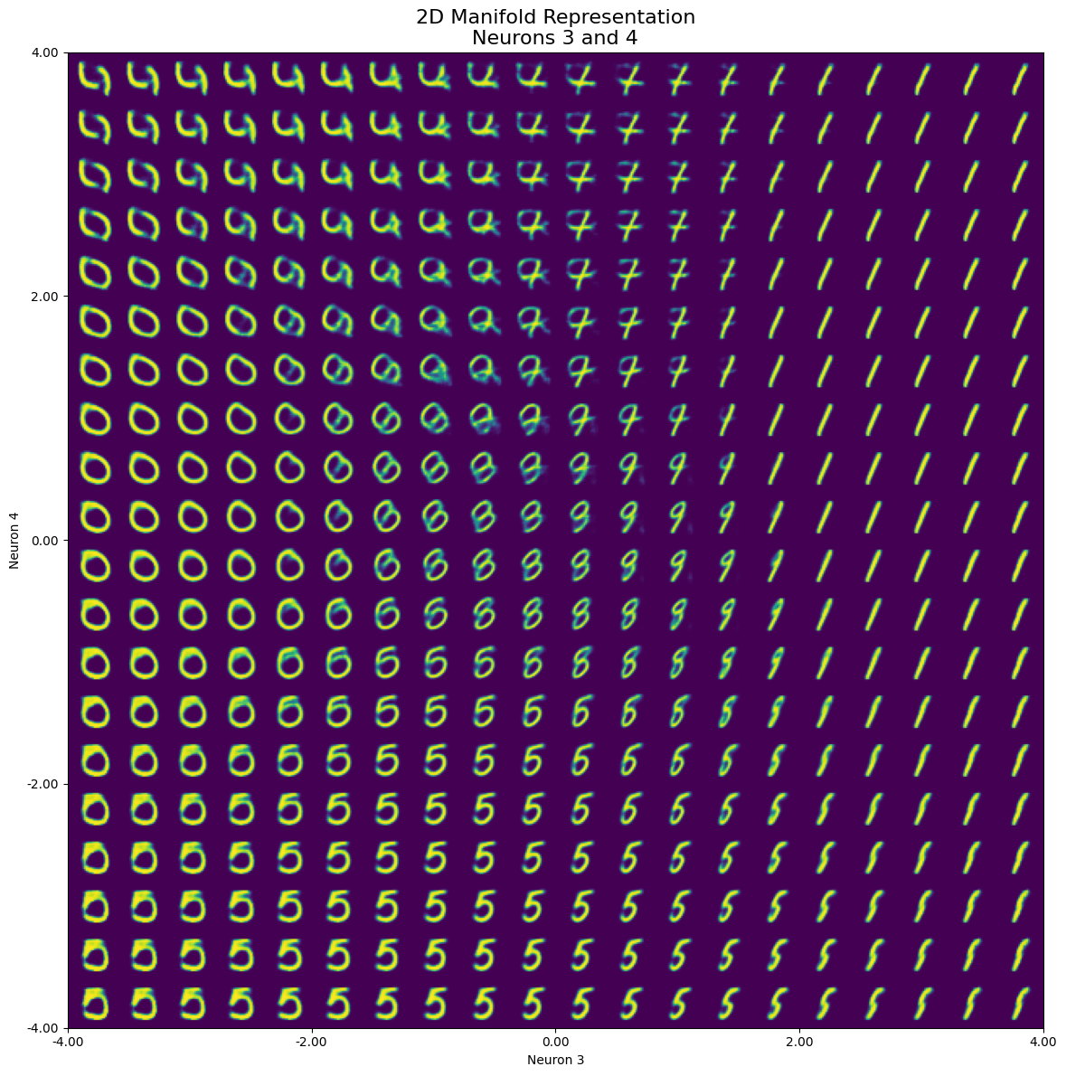
generate_2d_manifold(model, neuron1, neuron2, neuron_values, num_images=1, steps=20, start_value=start_value, end_value=end_value)
In the resulting image, we can observe that when iterating over both neurons simultaneously, only a small part of the set range actually represents our initial number 2. A limited range within the selected neurons is responsible for representing the “2”, while we see several other numbers such as 5, 0, and 1 (even with a small portion of 8 or 3) dominating the manifold space:
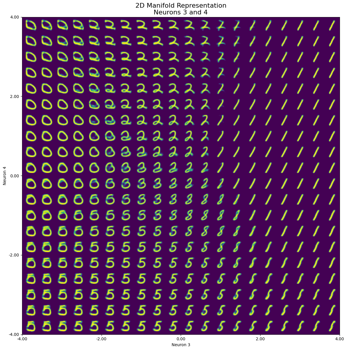
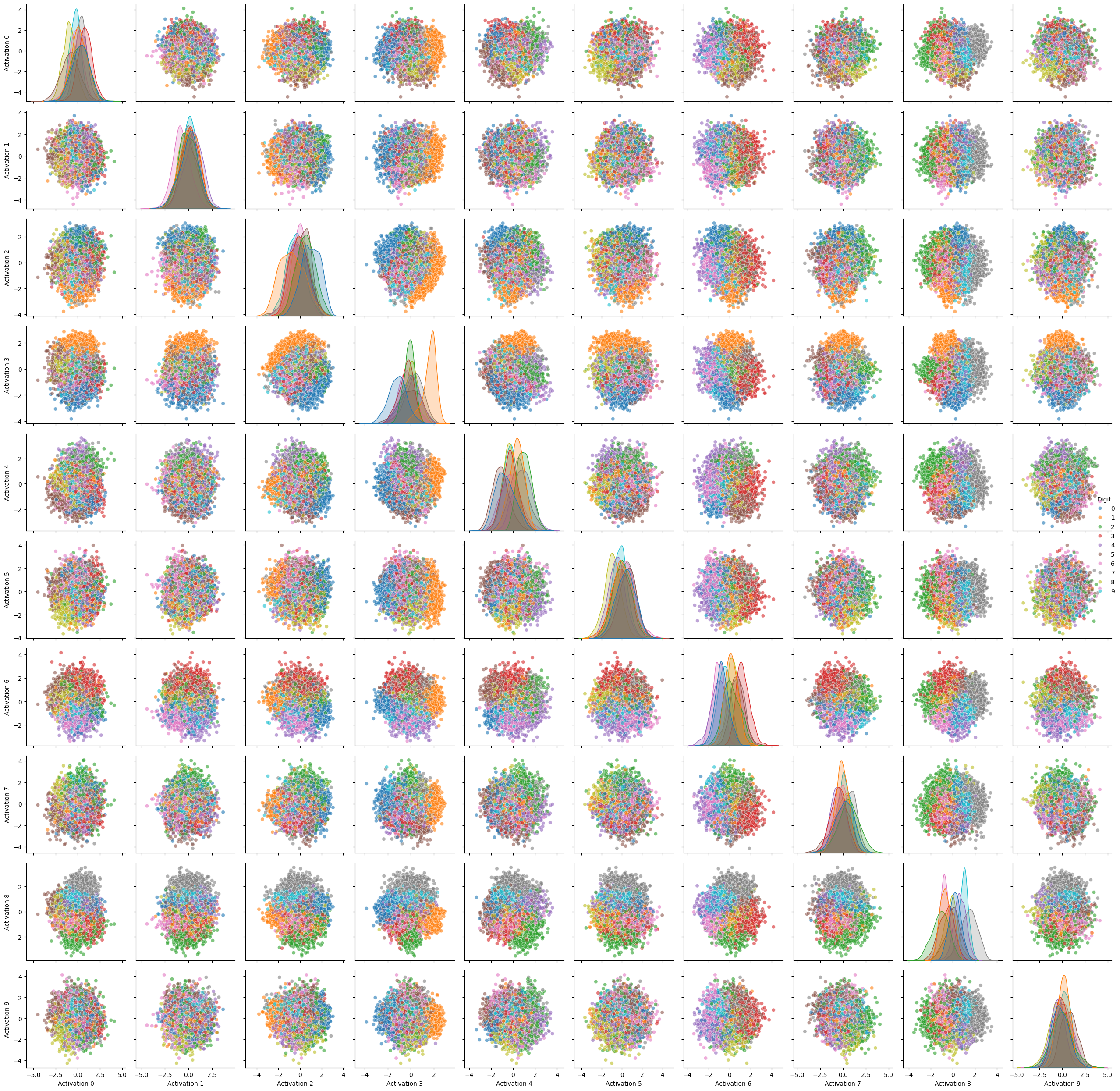
Furthermore, we can see the effect of “morphing” through a clockwise rotation from bottom to top (negative to positive values on neuron 4). This morphing results in different number shapes depending on the value of neuron 3. Another way to explore the latent dimensions is to make a grid of scatter plots for each pair of latent dimensions, color-coded by digit. The diagonal will show kernel density estimation plots for each dimension.
import matplotlib.pyplot as plt
import seaborn as sns
import pandas as pd
import numpy as np
from sklearn.preprocessing import StandardScaler

def create_pairwise_plots(df):
    # Extract latent representations
    latent_cols = [col for col in df.columns if col.startswith('Activation')]
    X = df[latent_cols].values
    y = df['Digit'].values

    # Standardize the data
    scaler = StandardScaler()
    X_scaled = scaler.fit_transform(X)

    # Create a DataFrame with scaled data
    latent_df = pd.DataFrame(X_scaled, columns=latent_cols)
    latent_df['Digit'] = y

    # Create a color palette based on 'tab10' colormap
    cmap = plt.get_cmap('tab10')
    unique_digits = np.unique(y)
    palette = {digit: cmap(i) for i, digit in enumerate(unique_digits)}

    # Create pairwise plots
    plt.figure(figsize=(20, 20))
    sns.pairplot(latent_df, hue='Digit', vars=latent_cols, diag_kind='kde', plot_kws={'alpha': 0.6}, palette=palette)
    plt.tight_layout()
    plt.show()

# Call the function
create_pairwise_plots(df)
Here we can clearly see which digit we can expect within certain coordinates of two corresponding neurons:
Now we can display the scatter plot for the neurons we visualized within our manifold representation:
import matplotlib.pyplot as plt
import pandas as pd
import numpy as np
from sklearn.preprocessing import StandardScaler

def visualize_selected_neurons(df, neuron1, neuron2, start_value=-4, end_value=4):
    # Extract latent representations
    activation_cols = [f'Activation {neuron1}', f'Activation {neuron2}']
    X = df[activation_cols].values
    y = df['Digit'].values

    # Standardize the data
    scaler = StandardScaler()
    X_scaled = scaler.fit_transform(X)

    # Create a DataFrame with scaled data
    plot_df = pd.DataFrame(X_scaled, columns=[f'Neuron {neuron2}', f'Neuron {neuron1}'])
    plot_df['Digit'] = y

    # Create the scatter plot

    plt.figure(figsize=(10, 8))
    scatter = plt.scatter(plot_df[f'Neuron {neuron2}'], plot_df[f'Neuron {neuron1}'], c=plot_df['Digit'], cmap='tab10')
    plt.title(f'Scatter Plot of Neuron {neuron1} vs Neuron {neuron2}', fontsize=16)
    plt.xlabel(f'Neuron {neuron1}')
    plt.ylabel(f'Neuron {neuron2}')
    plt.colorbar(scatter)

    # Set axis limits to match the manifold plot
    plt.xlim(start_value, end_value)
    plt.ylim(start_value, end_value)

    plt.tight_layout()
    plt.show()

# Select two neurons to visualize
neuron1 = 3
neuron2 = 4
start_value = -4
end_value = 4

# Call the function
visualize_selected_neurons(df, neuron1, neuron2, start_value, end_value)
Do you see the similarity with the manifold plot? Let’s compare them again and use zeros for default neuron values within the manifold plot:
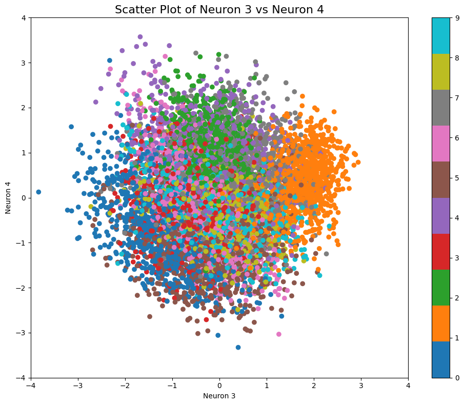
We can now clearly see how the number positions from the test subset scatterplot clearly correspond with the VAE generated images within the manifold representation.
Furthermore, based on the pairwise scatterplot, we can now visualize certain points of interest with VAE. We can use custom coordinates (as single value or list) or use line sampling with a set sample resolution (I set alpha=0.6 to make the sampling line more distinguishable):
import numpy as np
import matplotlib.pyplot as plt
from matplotlib.colors import BoundaryNorm
import matplotlib as mpl
from sklearn.preprocessing import StandardScaler
import torch
def sample_and_visualize_latent_space(df, model, device, neuron1, neuron2, sampling_points=None, line_start=None, line_end=None, n_line_samples=10):
# Extract latent representations
latent_cols = [col for col in df.columns if col.startswith('Activation')]
X = df[latent_cols].values
y = df['Digit'].values
# Standardize the data
scaler = StandardScaler()
X_scaled = scaler.fit_transform(X)
# Select the two specified neurons
X_selected = X_scaled[:, [neuron1, neuron2]]
# Define sampling points
if sampling_points is not None:
grid_points = np.array(sampling_points)
elif line_start is not None and line_end is not None:
grid_points = np.linspace(np.array(line_start), np.array(line_end), n_line_samples)
else:
raise ValueError("Either sampling_points or line_start and line_end must be provided.")
# Generate images from sampled latent points
model.eval()
with torch.no_grad():
# Create full latent vectors
sampled_latent_points = np.zeros((len(grid_points), X.shape[1]))
sampled_latent_points[:, neuron1] = grid_points[:, 0]
sampled_latent_points[:, neuron2] = grid_points[:, 1]
# Inverse transform the standardized data
sampled_latent_points = scaler.inverse_transform(sampled_latent_points)
latent_tensor = torch.FloatTensor(sampled_latent_points).to(device)
generated_images = model.decode(latent_tensor).cpu().numpy()
# Visualize generated images with coordinates
n_samples = len(grid_points)
n_cols = min(5, n_samples)
n_rows = (n_samples - 1) // n_cols + 1
fig, axes = plt.subplots(n_rows, n_cols, figsize=(2*n_cols, 2*n_rows))
fig.suptitle(f"Sampled Images from Latent Space (Neurons {neuron1} and {neuron2})", fontsize=16)
for idx, ax in enumerate(axes.flatten()):
if idx < n_samples:
ax.imshow(generated_images[idx].reshape(28, 28), cmap='viridis')
ax.axis('off')
coord = grid_points[idx]
ax.set_title(f"({coord[0]:.2f}, {coord[1]:.2f})", fontsize=8)
else:
ax.set_visible(False)
plt.tight_layout()
plt.show()
# Define colors for plotting
n_classes = len(np.unique(y))
cmap = plt.get_cmap('tab10')
norm = BoundaryNorm(np.arange(-0.5, n_classes + 0.5, 1), cmap.N)
# Plot latent space with sampling points
plt.figure(figsize=(10, 8))
scatter = plt.scatter(X_selected[:, 0], X_selected[:, 1], c=y, cmap=cmap, norm=norm, alpha=0.6)
plt.colorbar(scatter, ticks=np.arange(n_classes), label='Digit')
plt.scatter(grid_points[:, 0], grid_points[:, 1], c='black', s=50, marker='x')
if line_start is not None and line_end is not None:
plt.plot([line_start[0], line_end[0]], [line_start[1], line_end[1]], 'k-')
plt.title(f'Latent Space Visualization (Neurons {neuron1} and {neuron2}) with Sampled Points')
plt.xlabel(f'Neuron {neuron1}')
plt.ylabel(f'Neuron {neuron2}')
plt.show()
# Example usage:
# Assuming df is your DataFrame, model is your VAE, and device is your torch device
# Select two neurons to visualize
neuron1 = 3 # Change this to your desired neuron
neuron2 = 4 # Change this to your desired neuron
# # Option 1: Custom points
# custom_points = [
# [-2, 2], [-1, 2], [0, 2], [1, 2], [2, 2],
# [-2, 0], [-1, 0], [0, 0], [1, 0], [2, 0],
# [-2, -2], [-1, -2], [0, -2], [1, -2], [2, -2]
# ]
# sample_and_visualize_latent_space(df, model, device, neuron1, neuron2, sampling_points=custom_points)
# Option 2: Line sampling
line_start = [-1, -2]
line_end = [2, 1]
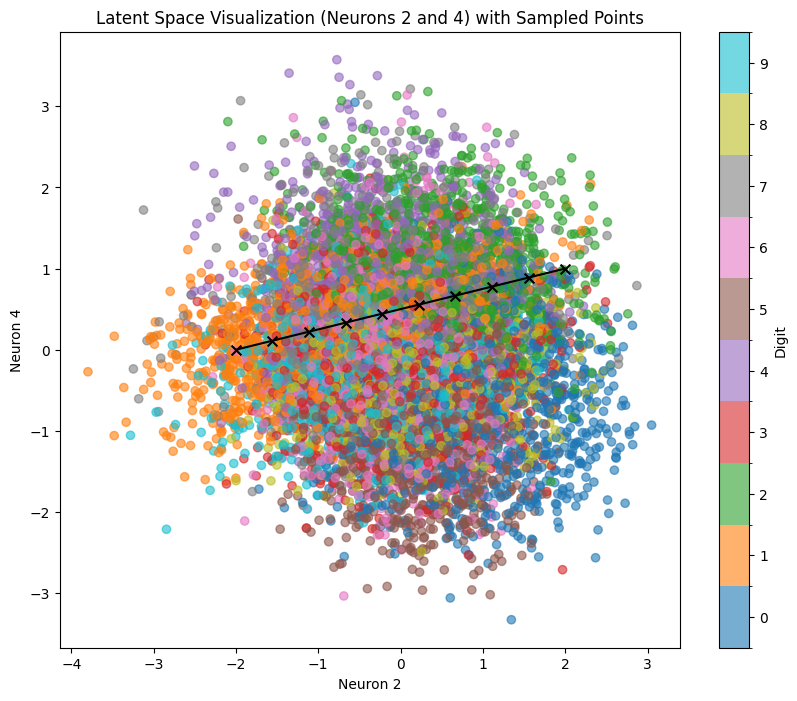
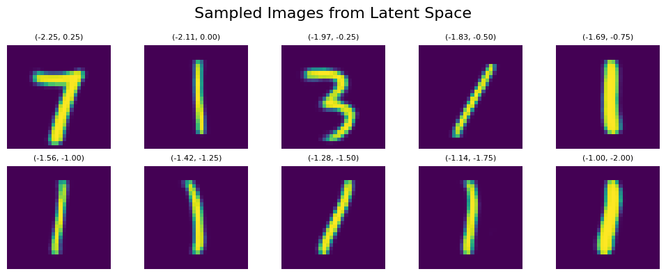
sample_and_visualize_latent_space(df, model, device, neuron1, neuron2, line_start=line_start, line_end=line_end, n_line_samples=10)
Here’s the corresponding output. Let’s sample across the line line_start = [-1, -2] line_end = [2, 1]
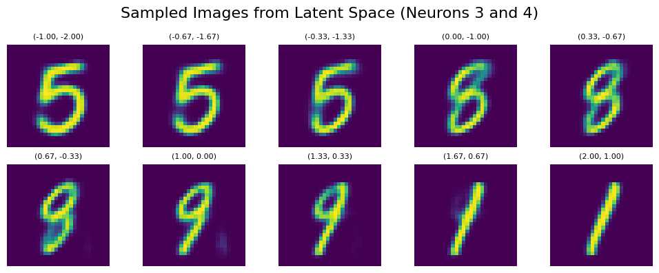
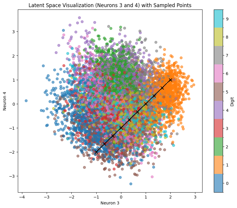
We can clearly see that despite sampling across areas with pretty clear number positions, we often get very blurry and deformed results because we are only activating 2 neurons out of 10 (other 8 are set to 0). To explore more complex relations that are representing all 10 available dimensions, we can use our test dataset with various dimensional reduction techniques.
Using t-SNE, PCA, and UMAP to Represent the Structure of Latent Space
t-SNE (t-Distributed Stochastic Neighbor Embedding), PCA (Principal Component Analysis), and UMAP (Uniform Manifold Approximation and Projection) are widely used in data analysis and visualization to uncover patterns and relationships within high-dimensional datasets. These techniques are particularly useful for various biology-related research tasks.
I won’t go into detail about these representations, as there are some excellent write-ups available:
- Dimension Reduction in Single Cell RNA-seq Analysis
- Towards a comprehensive evaluation of dimension reduction methods for transcriptomic data visualization
- Introduction to PCA, t-SNE and UMAP
- Visualizing MNIST: An Exploration of Dimensionality Reduction
In our case, we want to use all three representations to sample various points within the latent space. Let’s start with representations for our test dataset:
import numpy as np
import pandas as pd
import matplotlib.pyplot as plt
from sklearn.manifold import TSNE
from sklearn.decomposition import PCA
from umap import UMAP
from sklearn.preprocessing import StandardScaler

def plot_embedding(X, y, title):
    plt.figure(figsize=(10, 8))
    scatter = plt.scatter(X[:, 0], X[:, 1], c=y, cmap='tab10')
    plt.colorbar(scatter)
    plt.title(title)
    plt.xlabel('Dimension 1')
    plt.ylabel('Dimension 2')
    plt.show()

def create_visualizations(df):
    # Extract latent representations
    latent_cols = [col for col in df.columns if col.startswith('Activation')]
    X = df[latent_cols].values
    y = df['Digit'].values

    # Standardize the data
    scaler = StandardScaler()
    X_scaled = scaler.fit_transform(X)

    # t-SNE
    tsne = TSNE(n_components=2, random_state=42)
    X_tsne = tsne.fit_transform(X_scaled)
    plot_embedding(X_tsne, y, 't-SNE Visualization of Latent Space')

    # PCA
    pca = PCA(n_components=2, random_state=42)
    X_pca = pca.fit_transform(X_scaled)
    plot_embedding(X_pca, y, 'PCA Visualization of Latent Space')

    # Print explained variance ratio for PCA
    # print(f"PCA explained variance ratio: {pca.explained_variance_ratio_}")

    # UMAP
    umap_model = UMAP(n_components=2, random_state=42, n_jobs=1)
    X_umap = umap_model.fit_transform(X_scaled)
    plot_embedding(X_umap, y, 'UMAP Visualization of Latent Space')

# Assuming df is your DataFrame
create_visualizations(df)
It’s going to take a bit to calculate the representations, but we get 3 different representations:
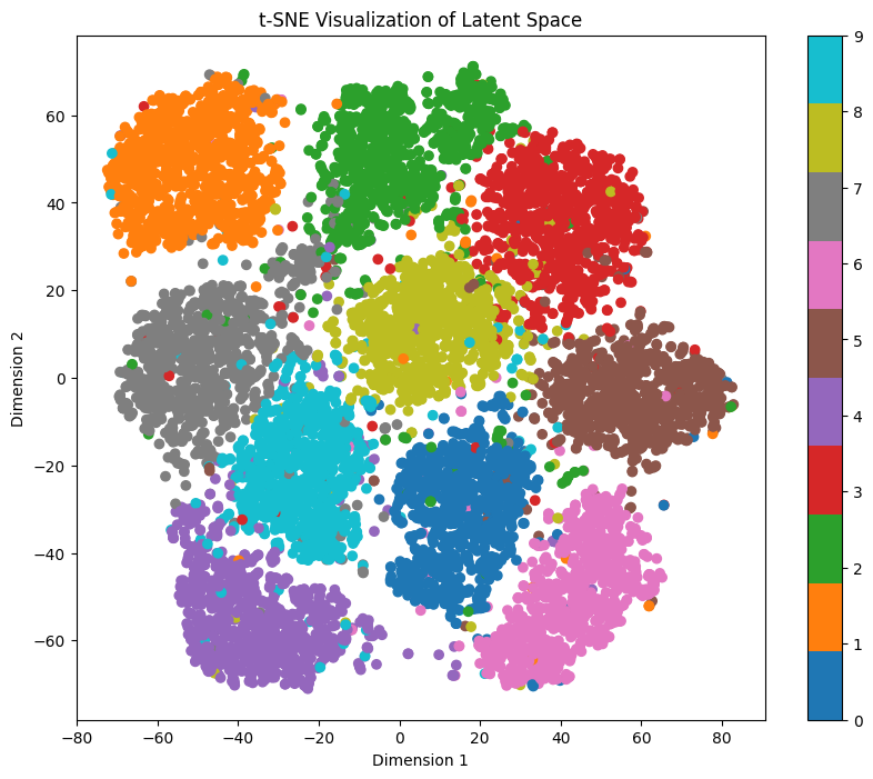
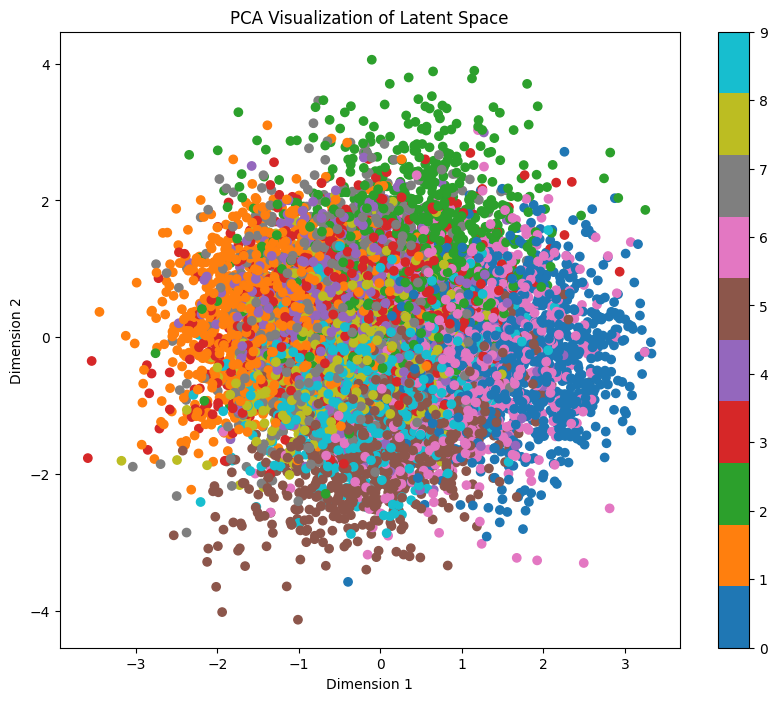
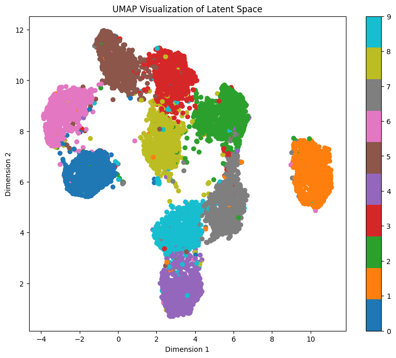
As we can see, each representation shows different entanglement features. While t-SNE and UMAP clearly show separation for each digit, PCA doesn’t. But wait, isn’t it looking very similar to our pairwise plot?
Let’s calculate the variance ratio for each principal component and visualize the loadings of the first two principal components:
from sklearn.decomposition import PCA
import matplotlib.pyplot as plt
import seaborn as sns
def analyze_pca_latent(df):
# Extract latent representations
latent_cols = [col for col in df.columns if col.startswith('Activation')]
X = df[latent_cols].values
# Perform PCA
pca = PCA()
pca.fit(X)
# Plot explained variance ratio
plt.figure(figsize=(10, 6))
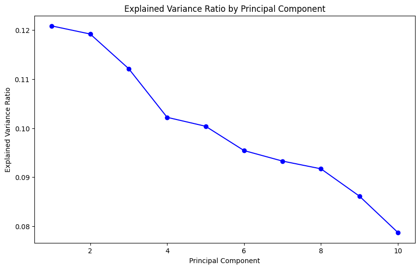
plt.plot(range(1, len(pca.explained_variance_ratio_) + 1), pca.explained_variance_ratio_, 'bo-')
plt.xlabel('Principal Component')
plt.ylabel('Explained Variance Ratio')
plt.title('Explained Variance Ratio by Principal Component')
plt.show()
# Plot loadings of first two principal components
loadings = pca.components_[:2, :]
plt.figure(figsize=(12, 5))
sns.heatmap(loadings, annot=True, cmap='coolwarm', yticklabels=['PC1', 'PC2'])
plt.xlabel('Latent Dimensions')
plt.title('PCA Loadings for First Two Principal Components')
plt.show()
print("Cumulative explained variance ratio:")
print(pca.explained_variance_ratio_.cumsum())
# Call the function
analyze_pca_latent(df)
Within PCA, it is to be expected that the first few principal components capture the most variance in the data, with each subsequent component capturing less:
But let’s take a look at loadings. By comparing the PCA loadings with pairwise plots, you can gain insights into how the original latent dimensions contribute to the principal components that capture the most variance in your data.
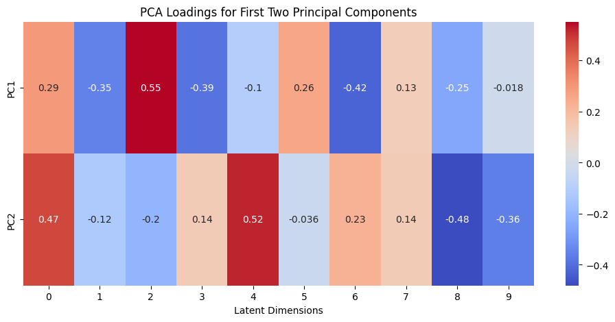
We can clearly see the importance of neurons 2 and 4. If we visualize the pairwise plot again with neurons 2 and 4, we see the following picture:
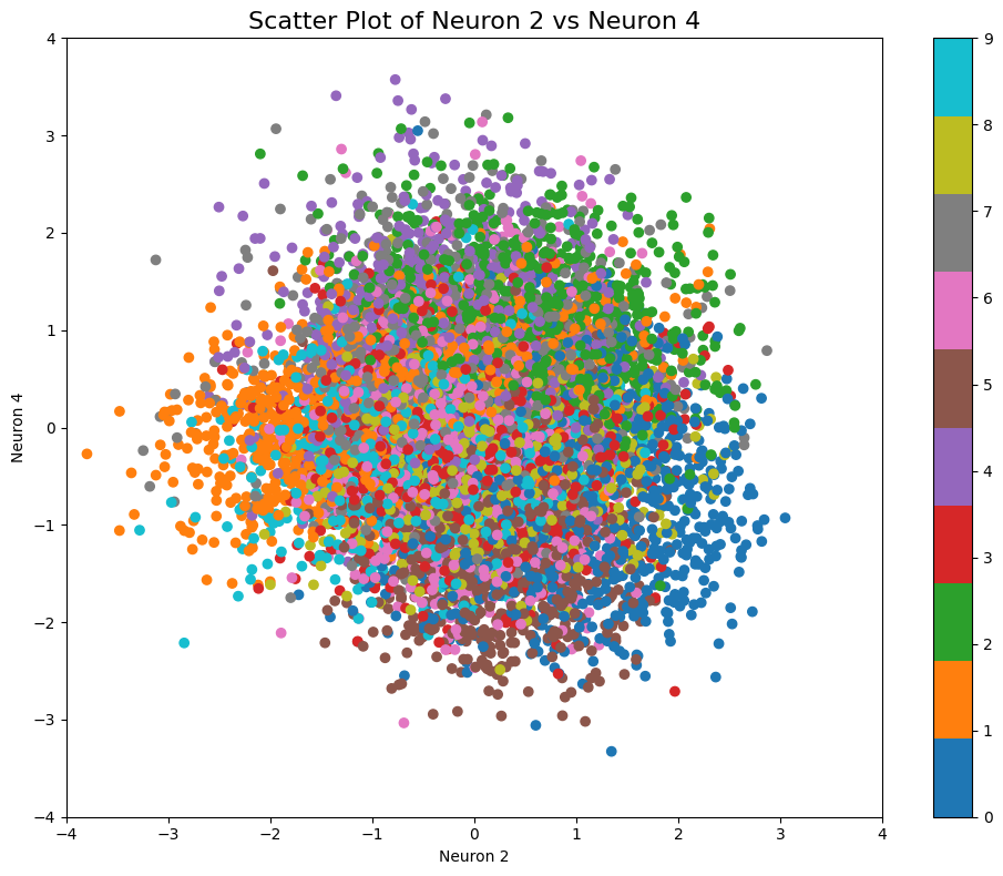
As expected, the spread of numbers within the pairwise plot looks very close to the PCA. But despite the similarity, if we now sample across the same coordinates, we can clearly see the big difference in output:
import numpy as np
import matplotlib.pyplot as plt
from matplotlib.colors import BoundaryNorm
import matplotlib as mpl
from sklearn.neighbors import NearestNeighbors
from sklearn.manifold import TSNE
from sklearn.decomposition import PCA
from umap import UMAP
import torch
import numpy as np
import matplotlib.pyplot as plt
from matplotlib.colors import BoundaryNorm
import matplotlib as mpl
from sklearn.neighbors import NearestNeighbors
from sklearn.manifold import TSNE
from sklearn.decomposition import PCA
from umap import UMAP
import torch
def sample_and_visualize_latent_space(df, model, device, method='umap', sampling_points=None, line_start=None, line_end=None, n_line_samples=10, print_values=False):
# Extract latent representations
latent_cols = [col for col in df.columns if col.startswith('Activation')]
X = df[latent_cols].values
y = df['Digit'].values
# Perform dimensionality reduction
if method == 'umap':
reducer = UMAP(n_components=2, random_state=42, n_jobs=1)
elif method == 'tsne':
reducer = TSNE(n_components=2, random_state=42)
elif method == 'pca':
reducer = PCA(n_components=2)
else:
raise ValueError("Method must be one of 'umap', 'tsne', or 'pca'")
X_reduced = reducer.fit_transform(X)
# Define sampling points
if sampling_points:
grid_points = np.array(sampling_points)
elif line_start and line_end:
grid_points = np.linspace(np.array(line_start), np.array(line_end), n_line_samples)
else:
raise ValueError("Either sampling_points or line_start and line_end must be provided.")
# Find nearest neighbors in reduced space
nn = NearestNeighbors(n_neighbors=1, metric='euclidean')
nn.fit(X_reduced)
_, indices = nn.kneighbors(grid_points)
# Get corresponding latent space points
sampled_latent_points = X[indices.flatten()]
# Optionally print the latent vector for each sampled point
if print_values:
for i, point in enumerate(grid_points):
neuron_values = {j: sampled_latent_points[i][j] for j in range(len(sampled_latent_points[i]))}
print(f"Selected Point: {point}")
print("neuron_values = {")
for key, value in neuron_values.items():
print(f" {key}: {value:.6f},")
print("}")
print("="*50)
# Generate images from sampled latent points
model.eval()
with torch.no_grad():
latent_tensor = torch.FloatTensor(sampled_latent_points).to(device)
generated_images = model.decode(latent_tensor).cpu().numpy()
# Visualize generated images with coordinates
n_samples = len(grid_points)
n_cols = min(5, n_samples)
n_rows = (n_samples - 1) // n_cols + 1
fig, axes = plt.subplots(n_rows, n_cols, figsize=(2*n_cols, 2*n_rows))
fig.suptitle("Sampled Images from Latent Space", fontsize=16)
for idx, ax in enumerate(axes.flatten()):
if idx < n_samples:
ax.imshow(generated_images[idx].reshape(28, 28), cmap='viridis')
ax.axis('off')
coord = grid_points[idx]
ax.set_title(f"({coord[0]:.2f}, {coord[1]:.2f})", fontsize=8)
else:
ax.set_visible(False)
plt.tight_layout()
plt.show()
# Define colors for plotting
n_classes = len(np.unique(y))
cmap = mpl.colormaps['tab10']
norm = BoundaryNorm(np.arange(-0.5, n_classes + 0.5, 1), n_classes)
# Plot reduced space with sampling points
plt.figure(figsize=(10, 8))
scatter = plt.scatter(X_reduced[:, 0], X_reduced[:, 1], c=y, cmap=cmap, norm=norm, alpha=0.6)
plt.colorbar(scatter, ticks=np.arange(n_classes), label='Digit')
plt.scatter(grid_points[:, 0], grid_points[:, 1], c='black', s=50, marker='x')
if line_start and line_end:
plt.plot([line_start[0], line_end[0]], [line_start[1], line_end[1]], 'k-')
plt.title(f'{method.upper()} Visualization with Sampled Points')
plt.xlabel('Dimension 1')
plt.ylabel('Dimension 2')
plt.show()
# Example usage:
# Assuming df is your DataFrame and model is your VAE
# Option 1: Custom points
# custom_points = [
# [-2, 1], [-2, 7], [0, 7], [2, 7], [4, 7],
# [-4, 0], [-2, 0], [0, 0], [2, 0], [4, 0],
# [-4, -7], [-2, -7], [0, -7], [2, -7], [4, -7]
# ]
# sample_and_visualize_latent_space(df, model, device, method='pca', sampling_points=custom_points, print_values=True)
# Option 2: Line sampling
line_start = [-2, 0]
line_end = [2, 1]
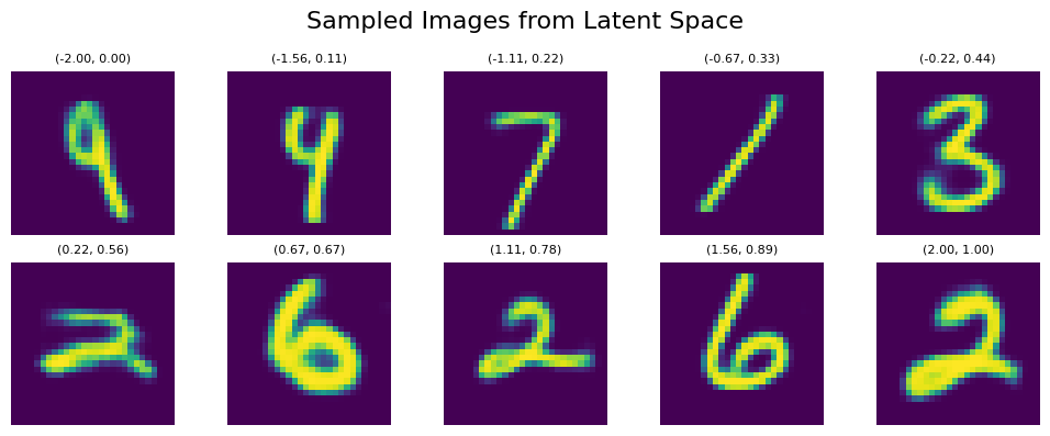
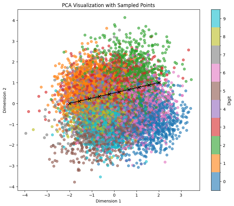
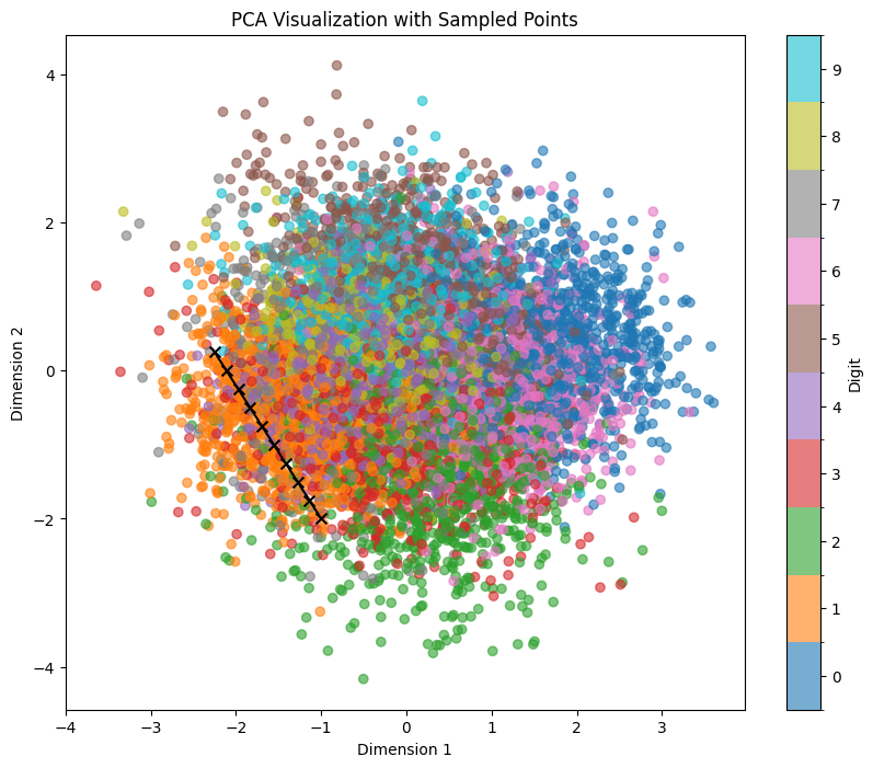
sample_and_visualize_latent_space(df, model, device, method='pca', line_start=line_start, line_end=line_end, n_line_samples=10, print_values=False)
And here’s the output:
Compared to sampling with similar coordinates in pairwise plot (neurons 2 and 4):
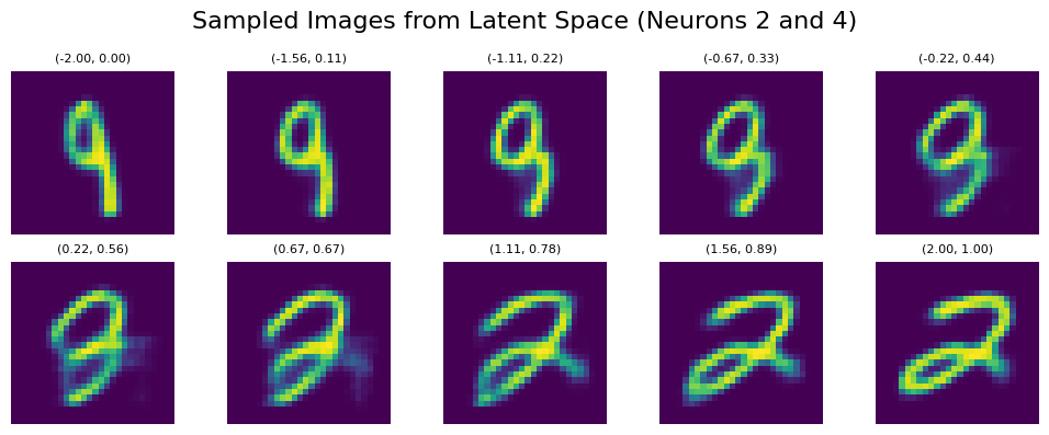
We can see that despite very similar sampling start and endpoints, the points in between within PCA clearly correspond to more complex points within the latent space. This way, even if we try to sample within a certain area where we expect to hit a certain number (e.g., if we try to sample 1 within the orange region in the example below), we are getting several false positives (other numbers). Also, we see that features like tilting or thickness aren’t clearly related to the x/y position of our sampling:
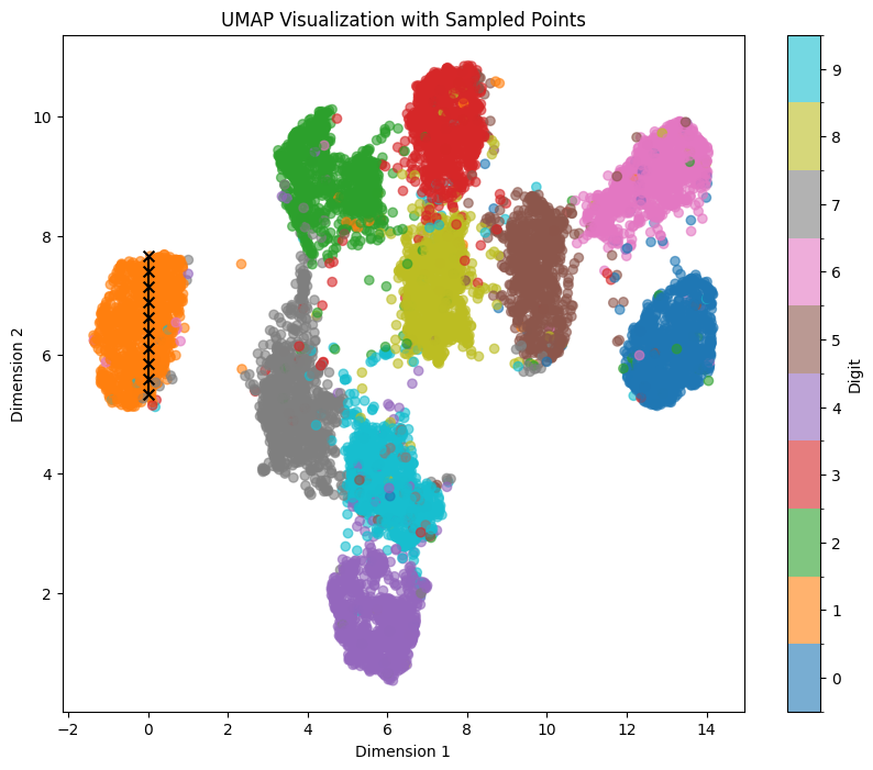
For exploring the latent space based on a specific digit while maintaining feature mapping within x/y dimensions, t-SNE and UMAP representations prove to be more suitable. In these representations, the numbers are distinctly separated from each other, although several clusters are densely packed.
Let’s sample the digit ‘1’ again within the UMAP representation, traversing a straight line from top to bottom within the orange area, using the coordinates line_start = [0, 7.66] line_end = [0, 5.33]:
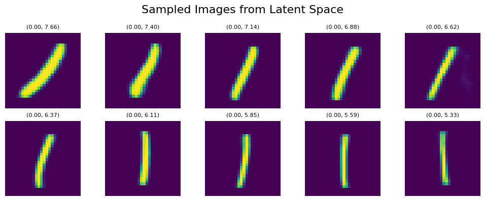
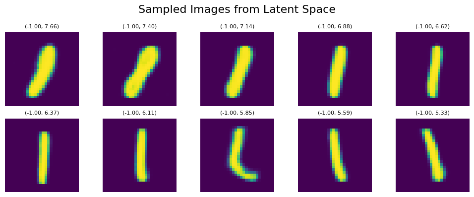
We can see clear affect of y value on both tilt and thickness of generated numbers. It persists even if we shift our sampling points within the x-Axis to the left with line_start = [-1, 7.66] line_end = [-1, 5.33]:

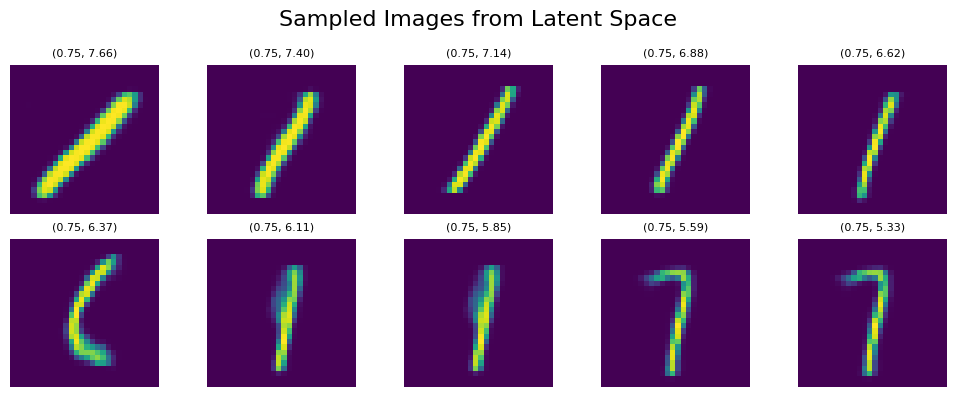
Similar behavior occurs if we shift our sampling points to the right to line_start = [0.75, 7.66] line_end = [0.75, 5.33]. However, if we leave the orange mapped area, some morphings to 7 start appearing as it’s the next nearest area to 1:

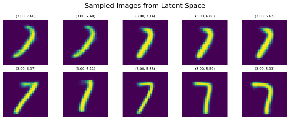
Interestingly, this behavior partially persists with rotation but without noticeable change in thickness even if we shift even further to the right, reaching the grey area (7) with line_start = [3, 7.66] line_end = [3, 5.33]:
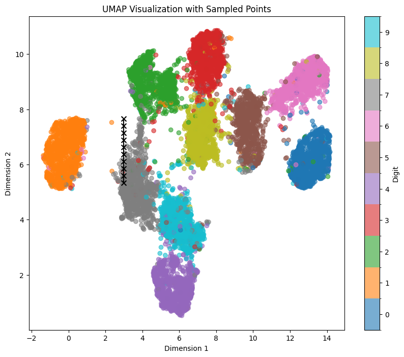
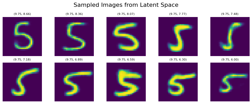
As we try similar sampling on other areas, we can clearly notice that features aligning with x/y axes clearly change depending on the number/area we are sampling. For example, if we try to sample the brown area with 5 vertically in a similar way with line_start = [9.75, 8.66] line_end = [9.75, 6], we clearly see another set of features (some kind of mixed morphing/rotation/thickness) aligned with the vertical axis:
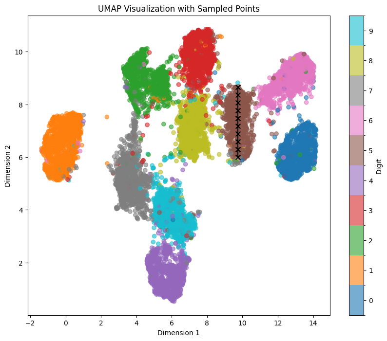
Here’s another example with number 0 and the blue area using line_start = [13, 7.25] line_end = [13, 5.25]:
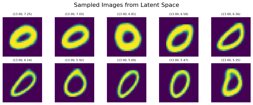

Although we see again some patterns containing thickness/rotation, it isn’t as well manifested as within digit ‘1’ and the corresponding orange area. However, overall we can still see the effect of position within the x/y axis on the generated output.
In case you want to find out what exact neuron values correspond to each sampled point, you can set print_values=True as a parameter within sample_and_visualize_latent_space function and get output in a similar format we used earlier for neuron progression and manifold representations:
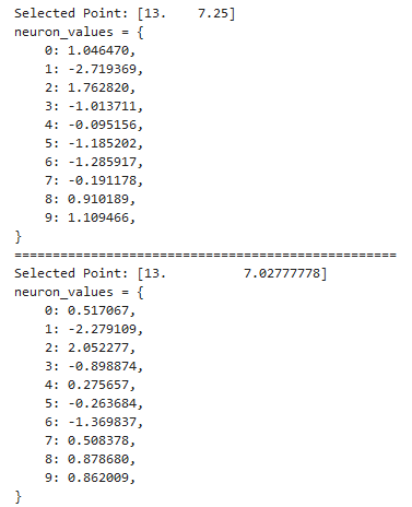
Just for reference, the t-SNE representation is somewhat similar to UMAP if we sample along the axes (usually t-SNE results in slightly bigger values for x/y axes), but the exact features and their variance, as well as dependence on x/y coordinates, may vary a lot in comparison with UMAP. Here’s an example of vertical sampling within the brown area (number 5) with line_start = [60, 18] line_end = [60, -17]:
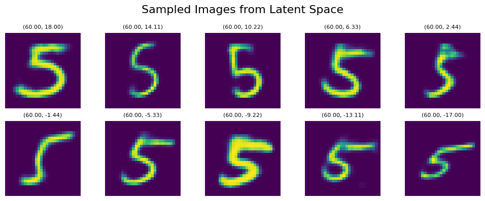
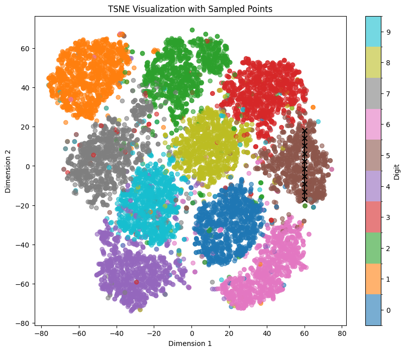
Interestingly, despite obvious differences in details, we are roughly getting similar features within our generated output. Especially the last 3 renders look very similar between UMAP and t-SNE! However, the deeper comparison between features represented in t-SNE and UMAP is a much broader topic that I’ll try to discuss in a separate post.
Some Closing Thoughts
Thank you if you read through the full post. It got much longer than I initially planned, but nevertheless, I think it might be useful for someone. During my personal study on this topic, I really missed some practical implementations for more or less “free” explorations of latent space based on different representations, especially dimension reduction-based algorithms like PCA, UMAP, and t-SNE. This need more or less determined the overall structure of the notebook and the features/methods I integrated into the code. Additionally, as I used this notebook in my classes, a lot of student feedback was integrated. I hope you find it helpful and enjoyable!
See you in the next blog!